
Hypothesizing about and measuring performance using the example of feature detection in computer vision.
Have you ever wondered how to learn most out of a performance measurement? Many developers rely solely on observing the measurement, but is there a more effective approach?
In this article, we will explore the concept of building a hypothesis for observed runtime behavior first, and then falsifying or confirming it via measurements. It is a more proactive and analytical approach that allows you to get more meaningful insights, because you thought about the problem theoretically first. Before we dive into the world of hypothesis-driven runtime measurements though, let us first look at the algorithm that we’ll be using as an example.
Almost every image processing pipeline does some sort of “feature” (think: object corner) detection. Such features can then be used to, e.g., track movement over several consecutive images. One algorithm for feature detection is the “Features from accelerated segment test” (FAST).
Features from Accelerated Segment Test (FAST)
For every pixel p in the image, we define a circle of 16 ordered pixels C (we call them “neighbors” although they are not directly adjacent to p). The circle is depicted in the following image:
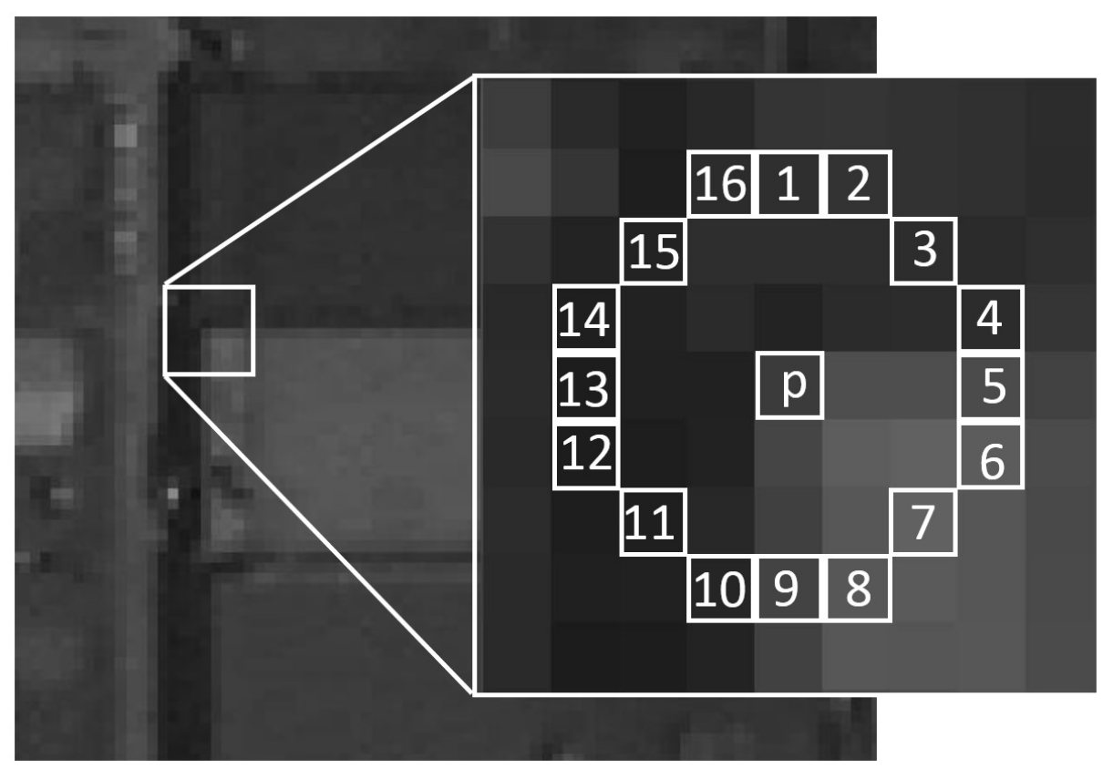
Illustration of the pixel neighborhood used in the FAST algorithm to determine if a pixel p is a corner. Image taken from: Huang, Jingjin, Guoqing Zhou, Xiang Zhou, and Rongting Zhang. 2018. “A New FPGA Architecture of FAST and BRIEF Algorithm for On-Board Corner Detection and Matching” Sensors 18, no. 4: 1014. https://doi.org/10.3390/s18041014 License: CC-BY.
The idea is to find contiguous segments on that circle that are either significantly darker or significantly brighter than the center pixel. In formal terms, pixel p is considered a feature, if and only if there exists a subset S of n contiguous (with respect to the order indicated by the numbers in the picture) pixels in C, so that either
- For all pixels q in S: I(q) > I(p) + t (dark corner), or
- For all pixels q in S: I(q) < I(p) - t (bright corner).
Here, I(p) is the intensity at pixel p and t is a detection threshold. Common choices for n are 9 or 12. Here, we use n=9. For more details about the algorithm itself, see this article on Wikipedia and the references therein.
Decision Trees
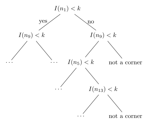
Illustration of the decision tree that fast-C-src uses. The neighbor luminosity values are denoted as I(.), k is the threshold luminosity, k = I(p) - t. Note: The illustration only shows the decision tree for bright corners and neglects the fact that the algorithm also checks dark corners. The actual implementation has two intertwined decision trees, one for “dark corner” condition and one for the “bright corner” condition.
For the FAST algorithm, one way to minimize the number of comparisons is to implement a binary decision tree. This is done in an implementation by Edward Rosten that you can find on GitHub. We call this implementation “fast-C-src” according to its repository name. Head over there for a second and scroll through the code to just get a glimpse of the implementation. The huge tree of if-else constructs should immediately catch your eye. The idea is closely related to an optimal game of Battleships: Choose the next comparison (among all 16 neighbors) that can potentially eliminate the most contiguous sequences of length n. A single decision tree for each pixel can be imagined as follows:
Test Setup: Raspberry Pi 3B+
To test how well this code performs, we need a well-defined execution environment, a level playing field that we use for all our measurements. All tests are performed on a Raspberry Pi 3B+. We configure it and our tools for maximum application performance.
The system details are:
- ARM Cortex-A53, 1 GB RAM
- CPU fixed at 1.4 GHz (Linux scaling governor: “performance”)
- Raspberry Pi OS 64 bit, Debian version 12 (Bookworm), Kernel 6.6.31
- Compilers: Debian 12 (Bookworm) default compilers for Arm64
- GCC 12.2 (Debian 12.2.0-14)
- Clang 14.0.6 (Debian 14.0-55.7~deb12u1).
- Compilation flags:
-O3 -mcpu=cortex-a53 -mtune=cortex-a53 -fno-stack-protector,--std=c11for C source files and--std=c++17for C++ sources - Google Benchmark version 1.9.0, release build
- glibc 2.36-9+rpt2+deb12u7
For the sake of simplicity, we use a single image for our tests:
This picture of a beautiful stream in the Wutach Canyon, which is located in the Black Forest (Baden-Württemberg, Germany).
We resize, crop and convert it to the PGM format using Imagemagick: convert input.png -resize 640 -crop 640x320 -depth 8 input.pgm.
This format is trivial to read in custom code.
We store the read data row-major as:
struct PGM {
  uint8_t *data;
  uint32_t xsize;
  uint32_t ysize;
};
After reading the PGM image, the measurement for fast-C-src is done with Google Benchmark:
void BM_fast_C_src_WithoutScoring(benchmark::State &state, PGM *pgm) {
  xy *corners;
  int num_corners;
  for (auto _ : state) {
    corners = fast9_detect(pgm->data, pgm->xsize, pgm->ysize, pgm->xsize, threshold, &num_corners);
    free(corners);
  }
}
💡 Note: Before measuring, always be clear about what to measure. Our small benchmark function measures the inverse throughput or frame time of the
fast9_detect. Thus, lower numbers indicate better performance.
The interface of fast-C-src returns a pointer with ownership. Internally, the function allocates memory for the result. We deliberately keep it that way.
💡 Note: Be careful when benchmarking library functions like malloc, free, etc. The variance of these functions can be high, because they can call into the kernel, have to deal with memory fragmentation, etc. We still include the calls in our benchmark because we want to use the unmodified original code.
Runtime: Clang beats GCC
If we build our test program with GCC and the flags mentioned above, this is the result:
$ taskset -c 1 ./testbench.GCC --benchmark_min_time=1000x --benchmark_repetitions=10 --benchmark_time_unit=ms
[...]
------------------------------------------------------------
Benchmark                  Time             CPU   Iterations
------------------------------------------------------------
[...]
fast-C-src_mean         8.34 ms         8.34 ms           10
fast-C-src_median       8.34 ms         8.34 ms           10
fast-C-src_stddev      0.002 ms        0.002 ms           10
[...]
The results show a very stable frame time of 8.34 milliseconds. Let’s run the same benchmark built with Clang:
$ taskset -c 1 ./testbench.CLANG --benchmark_min_time=1000x --benchmark_repetitions=10 --benchmark_time_unit=ms
[...]
------------------------------------------------------------
Benchmark                  Time             CPU   Iterations
------------------------------------------------------------
[...]
fast-C-src_mean         7.45 ms         7.44 ms           10
fast-C-src_median       7.44 ms         7.44 ms           10
fast-C-src_stddev      0.004 ms        0.003 ms           10
[...]
The Clang-built executable only takes 7.44 ms on average. This is 0.9 ms faster, or 11%. Apparently, Clang (namely its optimizer) produces binary code that performs faster on this particular input image.
💡 Note: With Profile-guided Optimization, we can make GCC produce executables that are on-par with Clang runtime-wise.
The interesting question is now: Why is that?
Of course, we could go ahead and compare the two binaries side-by-side.
That is not really feasible because the compiled machine code of fast9_detect from fast-C-src is about 13 kB, over 3000 instructions.
We need to find more efficient methods to determine what the difference is.
Fortunately, we can winkle out more information with measurements.
But first, let’s build a hypothesis!
Hypothesis: Better Tree Linearization
Even though the binary code is 13 kB, let’s still look at a small excerpt to understand how the compiler implements a tree if-else construct. It effectively needs to “cut” the tree into individual paths that can be laid out sequentially in memory. The other tree branches that diverge from this path are implemented as – surprise – branches. In this blog post, we call this a “linearization” of the tree. An excerpt of single path looks like follows:
# [...]
# This is the implementation of one tree node, or in code terms
# if (image[p + neighbor_offset[i]] < threshold) { ... } else { ... }
ldrb    w17, [x20, #4]
cmp     w17, w16
b.le    c184 <fast9_detect+0x394>
# This is another one
ldrb    w17, [x19, x18]
cmp     w17, w16
b.le    c314 <fast9_detect+0x524>
# And so on...
ldrb    w17, [x26, #6]
cmp     w17, w16
b.le    c500 <fast9_detect+0x710>
ldrb    w17, [x19, #6]
cmp     w17, w16
b.le    c7fc <fast9_detect+0xa0c>
ldrb    w17, [x28, #3]
cmp     w17, w16
b.le    cc50 <fast9_detect+0xe60>
# [...]
We see the implementation of 5 tree nodes.
The first instruction is always a load (ldrb) of a neighbor luminosity.
Then, it is compared (cmp) to the threshold in w16.
Based on this comparison, the following branch instruction either does nothing (if comparison evaluated to false) or it jumps to a given location (e.g. offset 0x394 from the start of the function).
This means, the instructions for one of the child nodes continue just below the parent’s implementation and the other child node is located somewhere else.
Both compilers produce equivalent code for a single tree node.
With this knowledge, we can build a hypothesis why the executable from Clang is faster: It could be due to the fact that Clang linearizes this tree differently, i.e. chooses to lay out different nodes sequentially. That could result in fewer nodes being traversed on average.
How can we test such a hypothesis? We can clearly see in the above disassembly, that each tree node is associated with a branch instruction. Also, we can count how many neighbor pixels on average we need to inspect.
💡 Note: In the following, we assume that the reader is somewhat familiar with Perf. For basic explanation of the output, consult the Perf Wiki, or an introductory book like Denis Bakhvalov’s “Performance Analysis and Tuning on Modern CPUs” over at easyperf.net.
Average Search Depth: How Deep do we Go in the Tree?
On suitable hardware, we can count taken branches or even every encountered branch instructions (including non-taken).
Fortunately, the Cortex-A53 supports both.
Let’s throw all branch-related events that perf list outputs at our program (these are: br_pred,br_mis_pred,branches,branch-misses,pc_write_retired).
$ perf stat -e instructions,br_pred,br_mis_pred,branches,branch-misses,pc_write_retired taskset -c 1 ./f9tb.cortex-a53.gcc --benchmark_min_time=1000x --benchmark_repetitions=1
[...]
     9,068,399,611      instructions:u
     2,153,337,047      br_pred:u
       545,863,367      br_mis_pred:u
     1,090,950,691      branches:u
       545,863,367      branch-misses:u                  #   50.04% of all branches
     1,090,950,691      pc_write_retired:u

       8.362193970 seconds time elapsed

       8.354324000 seconds user
       0.003999000 seconds sys
To understand the output, we must first understand that Perf has two different kinds of events.
The first one (listed second in perf list) are actual events that the underlying Performance Measurement Unit (PMU) of the CPU provides.
In our case, these are, e.g., br_pred, br_pred_mis and pc_write_retired.
Perf also defines some convenience names (like branches and branch-misses) that it internally derives from PMU events (the Perf tutorial calls them “monikers”).
This explains why in the output above, branches equals pc_write_retired and branch-misses equals br_mis_pred.
Events that are supported across all ARMv8-A CPUs are well-documented in the ARMv8-A Architecture Reference Manual, section D13.12.3.
The event pc_write_retired occurs when the program counter is changed by the software, i.e. taken branches.
The total amount of encountered branch instructions can be computed by summing br_pred + br_mis_pred, which gives 2,699,200,414.
Per pixel, that is: 2,699,200,414 / 1000 / 640 / 320 ≈ 13 encountered branch instructions.
But that includes all code, not only the tree traversal.
Other sources for branches in fast9_detect from fast-C-src include (non-exhaustive list):
- The loop over all pixels: For entry-controlled loops typically 1-2 branches per iteration.
- The check if the result array is large enough to hold another pixel, if a pixel turns out to be a corner.
So it is clear that the number of tree nodes traversed is smaller than 13, and likely smaller than 10. Even though, we cannot nail it down to a precise number, we can still use it for relative comparisons. Let’s take a look at the Clang-produced executable:
$ perf stat -e instructions,br_pred,br_mis_pred,branches,branch-misses,pc_write_retired taskset -c 1 ./f9tb.cortex-a53.clang --benchmark_min_time=1000x --benchmark_repetitions=1
[...]
     6,955,875,140      instructions:u
     2,178,559,626      br_pred:u
       543,540,671      br_mis_pred:u
       967,965,553      branches:u
       543,540,671      branch-misses:u                  #   56.15% of all branches
       967,965,553      pc_write_retired:u

       7.453869053 seconds time elapsed

       7.444271000 seconds user
       0.008000000 seconds sys
While the number of executed instructions is significantly lower, the total number of encountered branch instructions br_pred + br_mis_pred 2,722,100,297 is not.
Interestingly, the number of taken branches (pc_write_retired) is almost exactly 11% lower than for the GCC-produced executable.
This finding falsifies our hypothesis. If the overall number of branch instructions is the same, the number of visited nodes is likely the same. However, the lower number of taken branches points still indicates a better linearization, one where the control flow is more sequential (less jumping).
How Much Data do we Access?
Recall the disassembly from above. There, every tree node is associated with one load, the neighbor luminosity. Of course, the luminosity of the central pixel needs to be loaded as well.
Every regular (non-special) memory access starts at the top of the memory hierarchy, i.e. level 1 data cache (L1D$).
This means that we can count the number L1D$ accesses in order to count the total number of memory accesses.
We do this with the l1d_cache PMU event:
perf stat -e l1d_cache ./testbench.GCC --benchmark_repetitions=1 --benchmark_min_time=1x
With GCC, the result are the following:
| #Iterations | 10 | 100 | 1k | 10k |
|---|---|---|---|---|
| L1D$ accesses [in thousands] | 18,954 | 182,586 | 1,818,914 | 18,182,151 |
| L1D$ accesses per pixel and iteration | ~9.3 | ~8.9 | ~8.9 | ~8.9 |
This nicely demonstrates the effect of averaging. With only 10 iterations, the constant (w.r.t. the number of iterations) overhead of our setup is still measurable. Starting with 100, it seems to be averaged out almost completely, and we can see that this executable accesses about 8.9 values per pixel.
The Clang-built executable consistently has about 0.5 accesses per pixel less on average:
| #Iterations | 10 | 100 | 1k | 10k |
|---|---|---|---|---|
| L1D$ accesses [in thousands] | 17,954 | 172,584 | 1,718,848 | 17,181,520 |
| L1D$ accesses per pixel and iteration | ~8.8 | ~8.4 | ~8.4 | ~8.4 |
On average for a single pixel we access the pixel itself and 7.9 other values (8.9 values in total) for GCC and about 7.4 with Clang, before the result is known. Besides loading neighborhood values, the accessed values also contain writing the result, if a pixel turns out to be a corner. From this measurement, our expectation for the number of visited tree nodes on average should be 7-8.
From the branch count we know that both executables encounter about the same number of branch instructions, only the amount of taken ones diverges. Recall that the algorithm actually checks for dark and bright corners, so it has two intertwined trees. That means, the same neighbor pixel will pop up in multiple tree nodes. The Clang-built binary apparently re-uses more loaded pixel data. Half a pixel on average is not much. For that, it might suffice to re-use the loaded data for a single often visited node.
Conclusion
We saw that the executable built with Clang is about 11% faster and executes significantly fewer instructions (~20%). After looking at the disassembly, our hypothesis was that the tree linearization might be better suited for our input image.
It indeed is, but not as we hypothesized initially. We conducted two measurements: The branch count and the data access count. The number of branch instructions executed by both executables were the same, which indicated that it is not a tree with shorter paths (for our specific input image). Rather, our measurements pointed at the actual tree layout in code (number of taken branches) as well as data-reuse among different nodes.
Creating a hypothesis first required us to examine the actual binary and building a model of how the tree looks after it has been compiled into assembly. This is a crucial step, because it forces you to document your mental model; it makes it easy to see if that model was correct or not – much easier than if you just sought confirmation for measurement results once they are done.
Future Work
You might ask: “Can we do better?” Yes, we can. Currently, the Clang-built executable takes about 34 ns (or 50 clock cycles) per pixel. With vectorization, which is non-trivial in this case, you can get a factor of 5-7x faster.